Module 4: PID Control
This article is contained in Scilab Control Engineering Basics study module, which is used as course material for International Undergraduate Program in Electrical-Mechanical Manufacturing Engineering, Department of Mechanical Engineering, Kasetsart University.Module Key Study Points
- understand the basics of PID control
- learn the effects of 3 parameters to system response
- learn how response is degraded by integrator windup
- How to tune PID parameters by Ziegler-Nichols Frequency Domain method
Different forms of PID
The so-called “textbook” form of PID controller is described as follows This algorithm computes the control variable u as output, given the input e, the error between the command and plant output. We see that the control variable is a function of 3 terms: P (proportional to error), I (time integral of error), and D (derivative of error), with corresponding control parameters K (proportional gain), Ti (integral time), and Td (derivative time), respectively. Taking Laplace transform of (1), we have
 with the transfer function of PID controller
 Another common structure of PID algorithm is represented by
 In this form, the controller gains are distributed to each of the PID terms separately, with its transfer function
 For our discussion of PID controller, we focus on the form (4) and (5). Nevertheless, it is easy to convert between parameters of (1) and (4) by the relations
 Ex. 1: To get started with Xcos simulation of a PID feedback system, download file pid_feedback.zcos . This launches an Xcos diagram in Figure 1. This diagram can easily be constructed using Xcos standard palettes. It requires only a step_function, clock_c (from Sources palette), PID and CLR blocks (from Continuous time systems palette), SUMMATION (from Mathematical operations palette), MUX (from Signal Routing palette), and CSCOPE (from Sinks palette). The plant transfer function is a robot joint driven by DC motor model from module 1, with J = 10 and B = 1.
Figure 1 pid_feedback.zcos basic PID simulation diagram
Click on the Simulation Start button to see the step response. Try adjusting the PID gains and plant parameters to see their effects on the closed-loop system. PID parameter tuning is well studied in control engineering. Here we give a brief guideline. The proportional gain Kp is a dominant quantity that normally has some nonzero value. The integral gain Ki helps eliminate steady state error but too high value could introduce overshoot and oscillation. The derivative gain Kd could help the response to reach steady state faster but could amplify high frequency noise, and could affect stability if set too high. When the plant model is not known, adjusting these 3 gains to achieve good response could be problematic for an inexperienced user. Later we discuss a tuning procedure. Commercial PID controller products usually have auto-tuning functions for user convenience. Ex. 2: To experiment with the tracking and disturbance attenuation performance of PID control, we setup a feedback diagram in Figure 2.
Figure 2 PID feedback diagram
which can be constructed as an Xcos model pid_dist.zcos in Figure 3. The joint inertia and friction are set to J = 10 and B = 0.1, respectively. The step disturbance at the plant input is active at t = 2 sec, with step value of 80.
Figure 3 pid_dist.zcos Xcos model for PID feedback with disturbance
Note that in this example, we have the luxury of knowing the exact plant model. So it is possible to solve for a good set of PID gains. An approach used in [2] turns off the Ki gain first and solve for Kp and Kd that yields a critical-damped system at chosen natural frequency. Then Ki is adjusted to eliminate steady-state error. To elaborate, it is shown in [2] that when Ki is set to 0, the resulting second order closed-loop characteristic polynomial is described by which gives
 For example, suppose we select a critical-damped closed loop system \zeta = 1, with natural frequency \omega = 8. From (8), this yields Kp = 640 and Kd = 160. Table 1 below gives calculated P and D gain values for 3 selected natural frequencies.
| ω | Kp | Kd |
|---|---|---|
| 4 | 160 | 80 |
| 8 | 640 | 160 |
| 12 | 1440 | 240 |
Table 1 Kp and Kd gains for 3 different natural frequencies
Using these 3 sets of gain values, we simulate the step responses. The results are shown in Figure 4. As expected, the higher the natural frequency, the faster the response. We also see that the steady-state error from step disturbance cannot be eliminated with the PD controller.
Figure 4 step responses of PD control with disturbance d = 80
To fix this problem, we need to turn on the Ki gain of PID controller. With the controller transfer function described by (5), the closed-loop system is now of third order with the characteristic polynomial
 Applying Routh-Hurwitz criteria to (10), it can be concluded that, given all positive PID gains, the feedback system is stable if
 The same Xcos diagram in Figure 3 can be used by putting some positive integral gain in the PID block. Let us fix Kp = 1440 and Kd = 240, corresponding to natural frequency \omega = 8 rad/s. Figure 5 shows the responses from setting some values of Ki. We see that the steady-state error to command and disturbance is eliminated by increasing Ki, though higher value could introduce more overshoot.
Figure 5 step responses of PID control
Applying the bound (11) to this example yields This can be verified by setting Ki = 34575 . The oscillating response in Figure 6 shows that the closed-loop system is at the brink of stability.
Figure 6 closed-loop response at controller gains Kp = 1440, Ki = 34575, Kd = 240
Effect from Saturation
Analysis of PID feedback control is often performed under the assumption that the system is purely linear. In real devices, nonlinear elements emerge at certain points in the feedback loop. Saturation is one of them that could cause undesirable system response. This nonlinear effect normally results from physical limits of signals and system parameters, say, maximum motor torque and current. Another common saturation is the input limit of servo amplifier. An industrial servo amp might allow input voltage command in the range \pm 10 volts, for example. Effect from saturation is more pronounced when integral term is used in PID. The response could have excessive overshoot due to error accumulation in the integral term. This is known as integrator windup. See [1] for more detail. Ex. 3: To see an effect from input saturation, construct an Xcos model as in Figure 7, or download pid_ilim.zcos. It represents a comparison of two closed-loop systems, which are basically the same except that the lower one has its input bounded between \pm 50 units.
Figure 7 pid_ilim.zcos Xcos diagram for Example 3
The controller gains are set at Kp = 640, Ki = 1000, Kd = 160 . Running the simulation yields the step responses in Figure 8, and the control variables (controller output) in Figure 9. We see that input saturation causes significantly larger overshoot and also worsens disturbance response.
Figure 8 effect of integrator windup on output response

Figure 9 controller output with plant input limit
Tuning the PID Parameters
As stated before, adjusting the PID gains from scratch to achieve a good response may not be trivial. As a result, most commercial PID controllers have functions to tune the 3 parameters automatically. This is normally called “autotuning” feature. One of autotuning methods suggested in the literature makes use of some relay feedback mechanisms, which is closely related to a manual tuning scheme known as Ziegler-Nichols Frequency Domain (ZNFD) method. Hence we discuss this ZNFD scheme in the last part of this module. Note: The original ZNFD method applies the “textbook” PID equation (1). But since (1) and (4) are closely-related by (6), here we make a conversion so that standard PID block in Xcos, which assumes the form (4), can be conveniently used. To tune a PID controller manually by ZNFD method, follow this procedure- turn off both the integral and derivative terms; i.e., setting Ki = Kd = 0. So now the PID is left only with the proportional gain K. We crank K up to the point that the closed-loop system starts to oscillate. At this point, the plant output will swing in a constant sinusoid motion, not growing and not dying out. Write this value down on a paper as Ku.
- Measure the period of oscillation. Write it down as Tu.
- Use Table 2 to tune the controller parameters
| Controller Form | Kp | Ki | Kd |
|---|---|---|---|
| P | 0.5Ku | – | – |
| PI | 0.4Ku | 1.25Ku/Tu | -</td |
| PID | 0.6Ku | 2Ku/Tu | KuTu/8 |
Table 2: suggested PID parameters from ZNFD method
From the above procedure, we could observe a drawback of the basic ZNFD method: the system must oscillate at some point of gain setting before it becomes unstable. This implies the Nyquist plot must cross the negative real axis at some point. For the DC motor model we are using, the gain margin is infinity. Hence it is difficult to find the oscillating point and the Ku value. There is some trick to get around such limitation, but this is beyond the scope of this module. For our basic study, we simply modify the DC motor robot joint by adding some dynamics to it, so that the Nyquist plot of L(j\omega) crosses the negative real axis. Ex. 4: Let us assume that the PID output is passed through a LPF with cutoff frequency 500 Hz before feeding the plant input. Using the filter design guide from module 1, we have the LPF transfer function as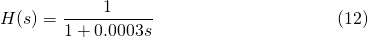 To simulate, construct an Xcos model in Figure 10, or download pid_znfd.zcos. With this model, we are ready to perform the ZNFD tuning procedure described above. Click on the PID block to set the I and D gains to zero. Then start increasing the P gain until the output oscillates. This is what you must do in a real application when the plant model is not known.
Figure 10 pid_znfd.zcos Xcos diagram for ZNFD tuning method
Well, in this example we do know the plant model, don’t we? So, to save us some time, the Ku value that causes output oscillation can be found, for example, using the method from Module 2. First from the loop transfer function containing the plant, LPF, and PID controller with Kp = 1.
-->kp = 1;
-->ki = 0;
-->kd = 0;

-->s=poly(0,'s');
-->P=syslin('c',1/(10*s^2+0.1*s));  // plant
-->H = syslin('c',1/(1+0.0003*s));  // filter
-->C=syslin('c',kp + ki/s + kd*s);  // controller
-->L = C*H*P; // loop t.f
Then find the gain where the closed-loop pole touches the j\omega axis.
->[kmax,s]=kpure(L)
 s  =
    5.7735027i
 kmax  =
    333.33433
resulting in Ku = 333.
Verify this by setting the P gain to 333 in PID block. This yields the desired oscillatory response as shown in Figure 11. The oscillation period can be roughly measured from the plot to yield Tu = 1 sec.
Figure 11 oscillatory response with Kp = 333, Ki = Kd = 0
So from the last row of Table 2, ZNFD method suggests the three PID parameters as Setting these gains gives the response in Figure 12.
Figure 12 response from PID gains suggested by ZNFD method
Note that the overshoot is quite excessive (70%). In a sense, ZNFD just gives us some good values to start with. We may want to fine-tune the PID gains to improve the response further. For example, decreasing the Ki gain would bring the overshoot down. Figure 13 shows the response from original PID gains (green), compared with the case when Ki is reduced to 300 (blue), and 200 (magenta).
Figure 13 reduce overshoot in the response by decreasing Ki
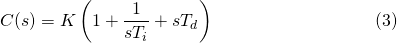
The ZNFD method could be explained using a Nyquist diagram in Figure 14. The diagram shows how a point x on the curve is moved related to the P, I , and D terms. Using the P term alone, x could be moved in radial direction only. The I and D terms help provide more freedom to move perpendicular to the radius. It can be shown that by using ZNFD method, the critical point (-1/Ku, 0) is moved to the point -0.6 – 0.28i. The distance of this point to the critical point is 0.5. So the sensitivity peak is at least 2. This explains the high overshoot in the step response.
Figure 14 How a point on Nyquist curve is moved with PID control
Summary
PID is a simple control structure that is still used widely in various industrial applications. It is a close relative to the lead-lag compensator explained in module 2, except that its functionality may be more user-friendly. With some knowledge and practice, an engineer or technician would be able to tune and operate a plant equipped with PID control. In this module we discuss the basics of PID feedback systems, with emphasis on Xcos simulations to show how the responses are related to three control parameters, as well as effect from input saturation that could worsen the response. Without some good starting values, tuning the PID gains can be cumbersome for a novice. So at the end, we mention a manual tuning procedure known as the Ziegler-Nichols frequency domain method. Some auto-tuning scheme of a commercial PID controller, such as the relay feedback method, is based on the ZNFD manual tuning.References
- K.J. Astrom and T.Hagglund. PID Controllers, 2nd ed., Instrument Society of America, 1995.
- M.W.Spong, S. Hutchinson and M. Vidyasagar, Robot Modeling and Control. John Wiley & Sons. 2006.
- V. Toochinda. Digital PID Controllers, 2009.
- V.Toochinda. Robot Analysis and Control with Scilab and RTSX. Mushin Dynamics, 2014.
